Overview
MacroBase provides a range of functionality, including exploratory data analysis and specialized operators for data types including time-series and streaming data. The easiest way to interact with the system is via the exploratory GUI, which we describe below. Most of the advanced functionality hasn't yet made its way to the GUI, so the best way to access it is by emailing us or poking around the repo.
To build and start the GUI server
- Clone the repo:
git clone https://github.com/stanford-futuredata/macrobase.git - Build MacroBase:
cd macrobase; mvn package- Note: after the first build,
mvn compileshould be sufficient. - Note: if you update pom.xml, you can also run
mvn dependency:copy-dependenciesinstead ofmvn package. - Note: your IDE should have an option to import an existing Maven project. Point the import tool at
macrobase/pom.xml.
- Note: after the first build,
- Load some data. Set up a postgres server on localhost with a database named
postgres. Then runpython tools/load_demo.py. - Note: to manually inspect the data:
psql postgresthen run\d sensor_data_demo;orSELECT * FROM sensor_data_demo LIMIT 10; - Start the MacroBase server:
bin/frontend.sh - Connect to the GUI: Open http://localhost:8080/ in your browser.
Common issues
- postgres username / password: edit conf/macrobase.yaml and set the parameters macrobase.loader.db.user and macrobase.loader.db.password
- data loading issues: try using a csv. See https://github.com/stanford-futuredata/macrobase/wiki/Running-MacroBase-Queries
MacroBase Exploratory GUI
- Configure the data source. MacroBase pulls data from a view defined by the 'Base Query' field. For our demo data, set 'Base Query' to
SELECT * FROM sensor_data_demo;and presssubmit.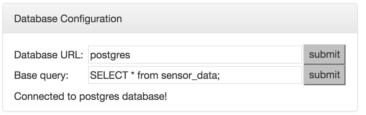
- Explore some sample data. You can explore a sample of the data by pressing
sample.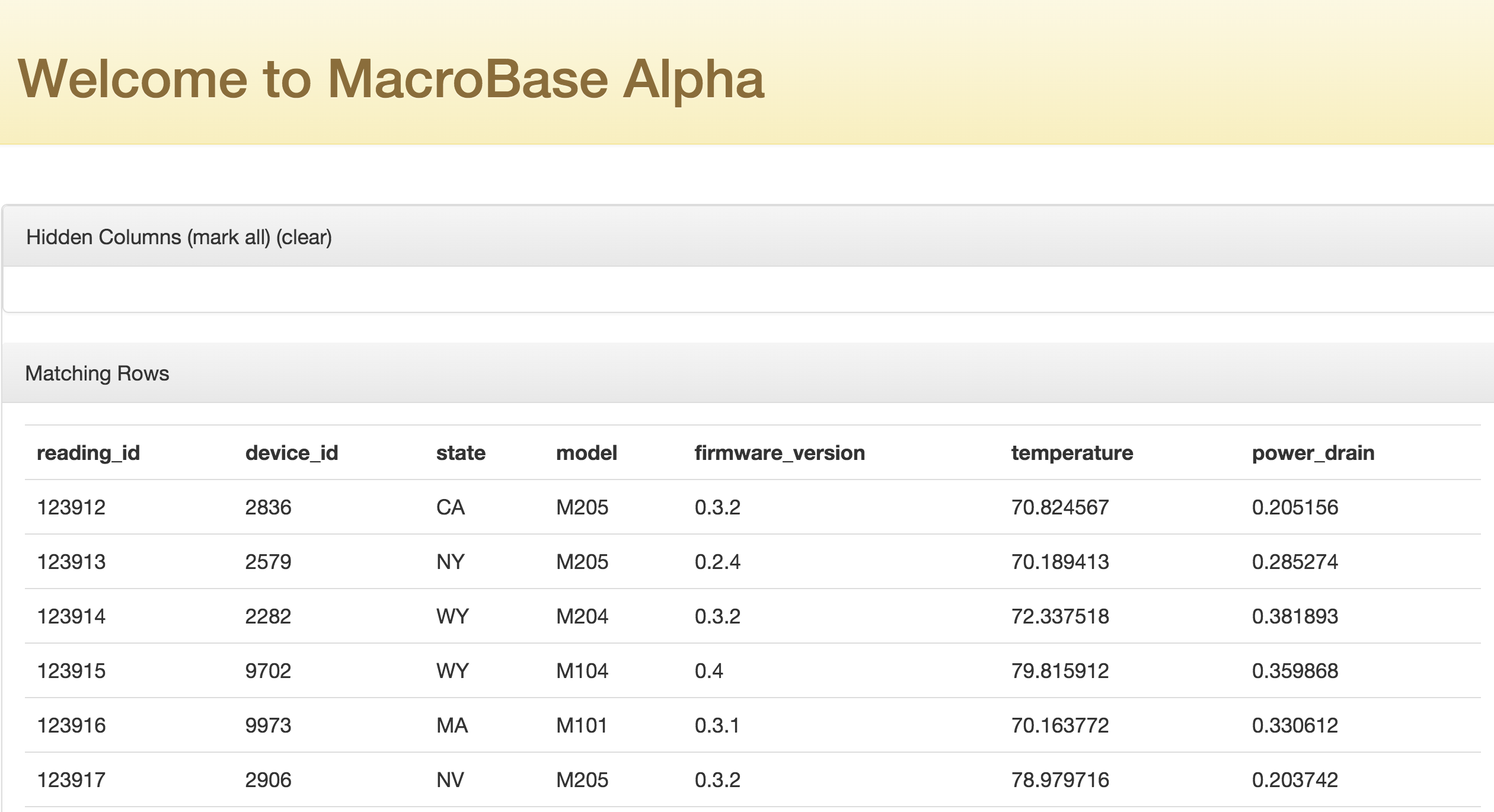
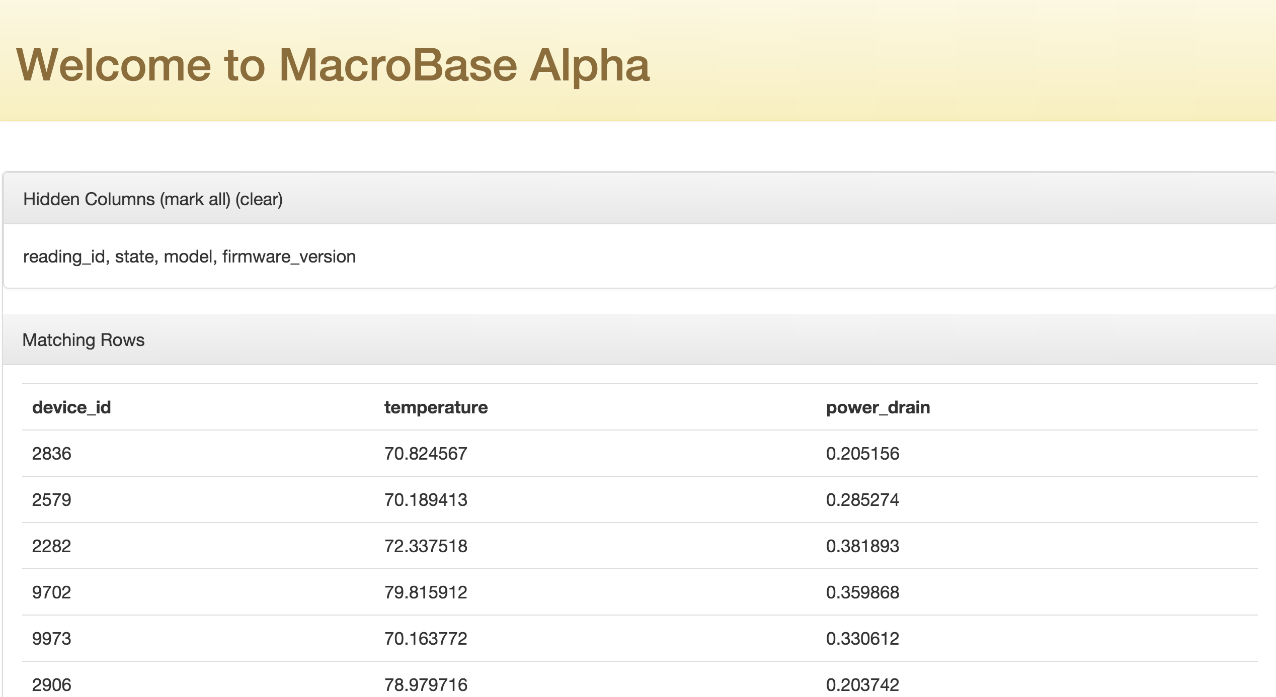
- Note: you can hide columns by clicking on their header name, or unhide them by clicking on their names in the 'Hidden Columns' list. You can hide all columns by clicking 'mark all' and unhide all by clicking 'clear'.
- Note: you can fetch more rows by clicking 'more rows' at the bottom of the page.
- Select columns for analysis. Let's say we want to find sensors with high power drain. We first select the 'power drain' column and mark it as a "Hi" 'Target Metric' by clicking the corresponding up arrow. We can correlate readings with high power drains with other attributes. Select the 'device_id', 'state', 'model', and 'firmware_version' columns as "Clustering Attributes" to correlate with by clicking the corresponding "+" button. Your screen should look like this:
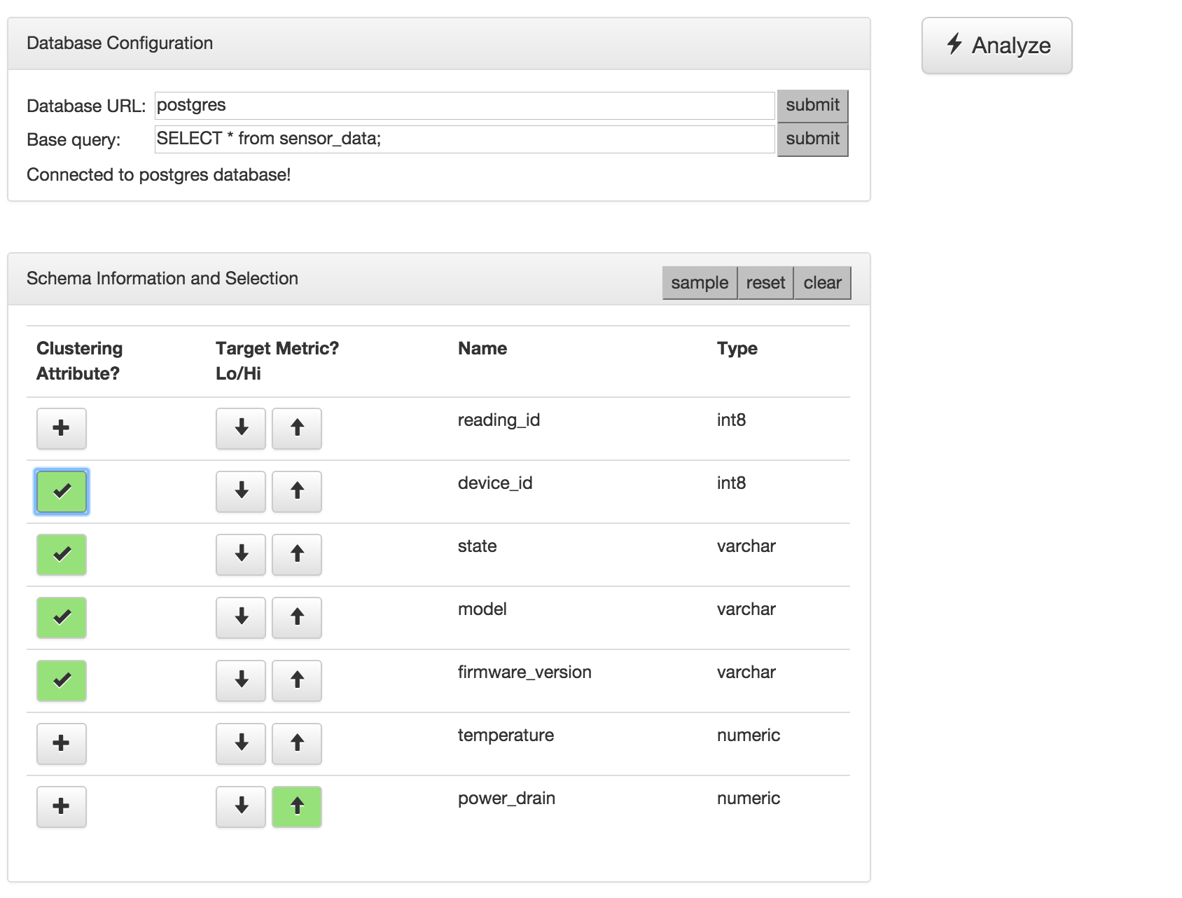
- Note: currently, we limit clustering attributes to categorical data (i.e., anything that would work for an enum type) instead of looking at continuous values (e.g., any points within a 50 mile radius of a given data point).
-
Note: we also require users to specify which attributes and metrics they are interested in, as well as which metrics are low and high. In the future, we can consider automatically suggesting "interesting groupings" for users.
-
Perform analysis. Click the 'analyze' button. In a few seconds, you should see your results below, like this:
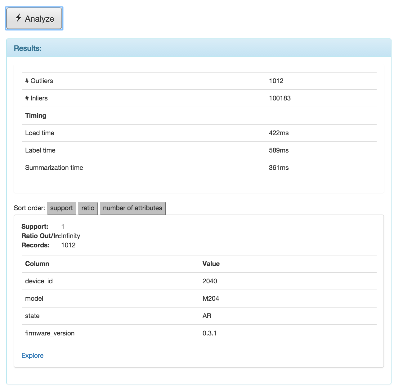
What we see is that we found 1012 records with high power drain readings. The list below shows attribute-value combinations that were highly correlated with high power drain readings; in this scenario, we only found one group: (device_id = 2040, model = M204, state = AR, firmware_version = 0.3.1).
-
What do the statistics mean?
- Support is the proportion of records marked as outliers that contained this attribute combination. Theoretical minimum is 0 (no outliers had this pattern), maximum is 1 (all outlier records matched).
- Ratio Out/In is the proportion of outlier records containing this attribute combination compared to the proportion of inlier records containing this attribute combination (i.e., support in outliers divided by support in inliers). A ratio of 1 means that this pattern appeared equally frequently in inlier and outliers. A ratio of infinity means this pattern was not present in the inliers.
- Records is the actual number of outlier records matching this pattern (i.e., support * number of outliers).
-
Note: you can explore records matching each combinations by clicking the corresponding 'Explore' link.
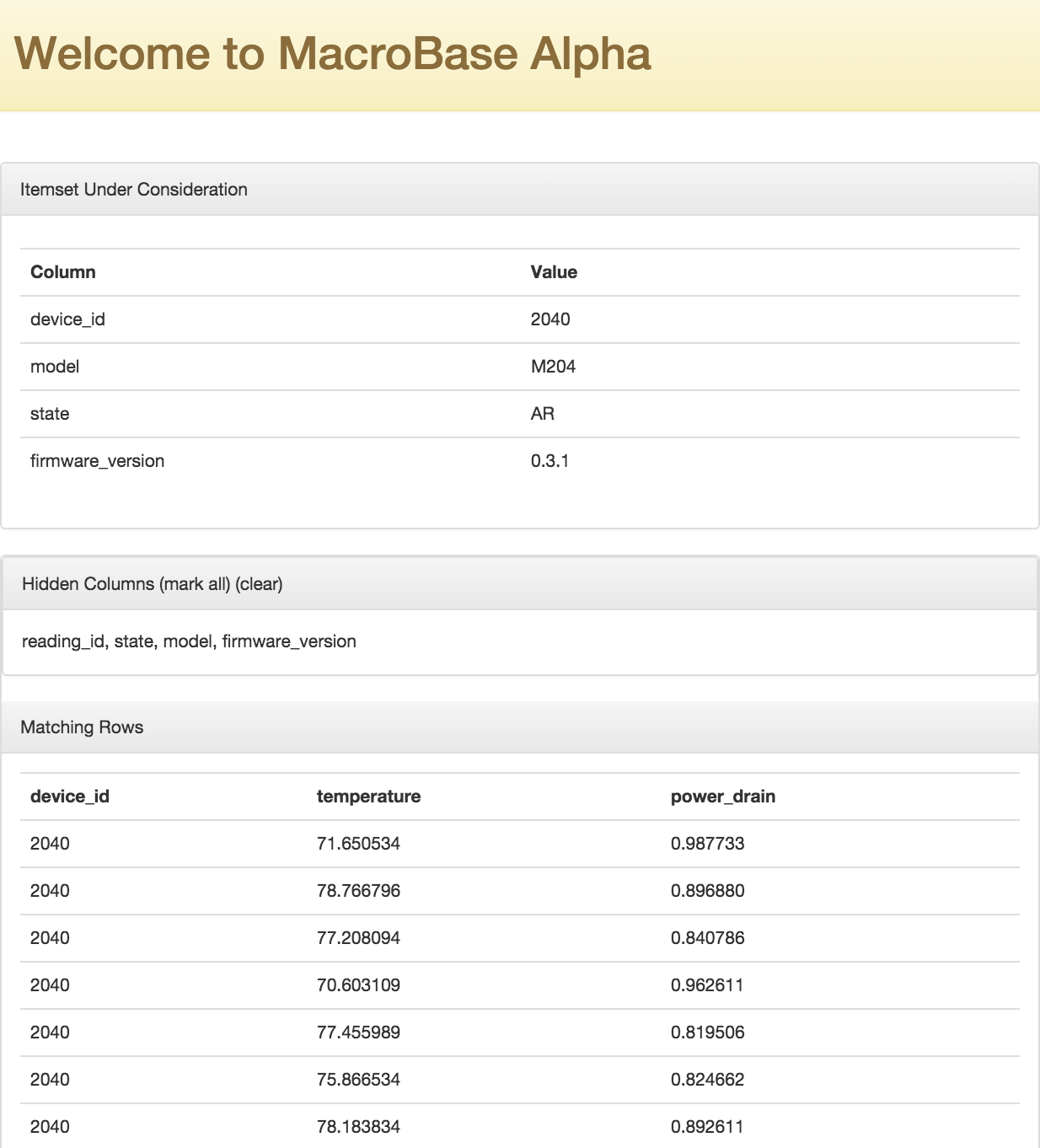
Can you tell why these these records marked as outliers?
-
Note: in the future, we'd like to add histograms to the summary screen so that it's more clear why records are marked as such as well as how they differ from the inlier distribution.
-
Try it yourself. Repeat the analysis to find records with low temperature readings.
- Note: you can also try finding multiple metrics of interest at once.
MacroBase Command Line
- Running batch analysis:
bin/batch.shrepeats the above, but using a pre-configured set of tables and columns. The configuration is stored inconf/batch.yaml. You likely need to editbatch.yamlto work for thesensor_data_demodataset. -
Note: you can change the configuration file!
batch.shis just a thin wrapper formacrobase.MacroBase batch <CONFIG_FILE> -
Running streaming analysis:
bin/streaming.shperforms a similar task using a one-pass streaming algorithm. There are considerably more parameters here to explore. - Note: again, you can change the configuration
macrobase.MacroBase streaming <CONFIG_FILE>